Example 2: Consider the system
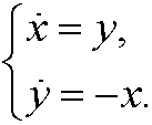
If we differentiate the first equation on time we get
that inserted into the second implies that
This differential equation has the solution

for some constants a and b. Since y is the derivative of x we have

Finally we note that
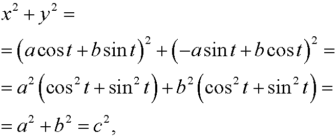
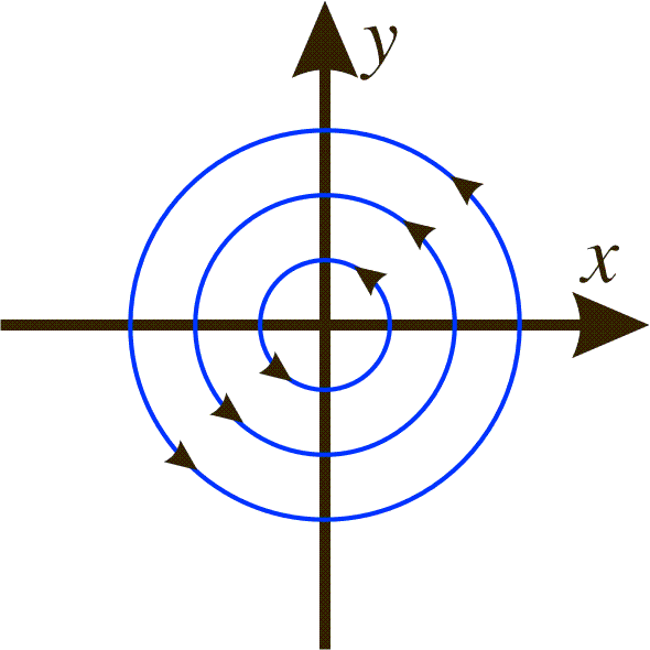
where c is a constant. The only equilibrium point obviously is (0,0). The phase portrait looks like this:
Remark: The relation x2+y2=c2 may also be obtained in the following way:
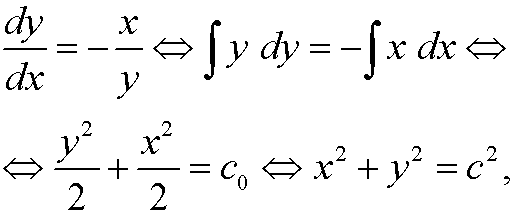
where

Example 3: Consider the system
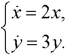
This decoupled system has the solution
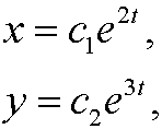
where c1 and c2 are two arbitrary constants. To draw the phase portrait we solve the equation
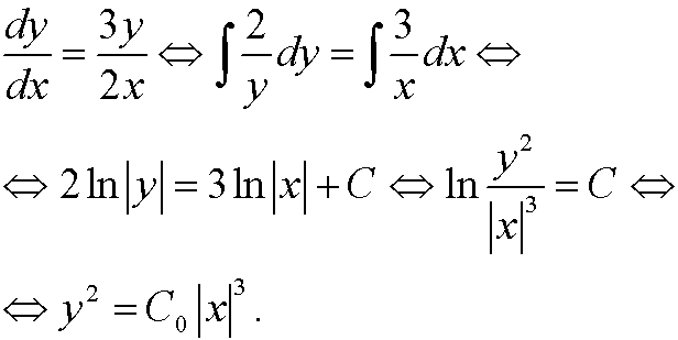
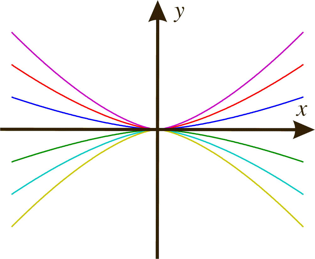
The phase portrait thus becomes:
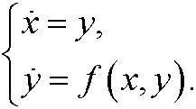
Example 4: Every second order differential equation

can be written as a system of first order differential equations
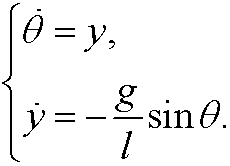
Example 5:

can be written as the system
We get the equilibrium points when
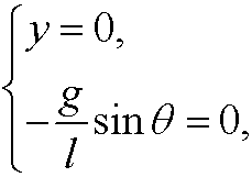
that is, they are

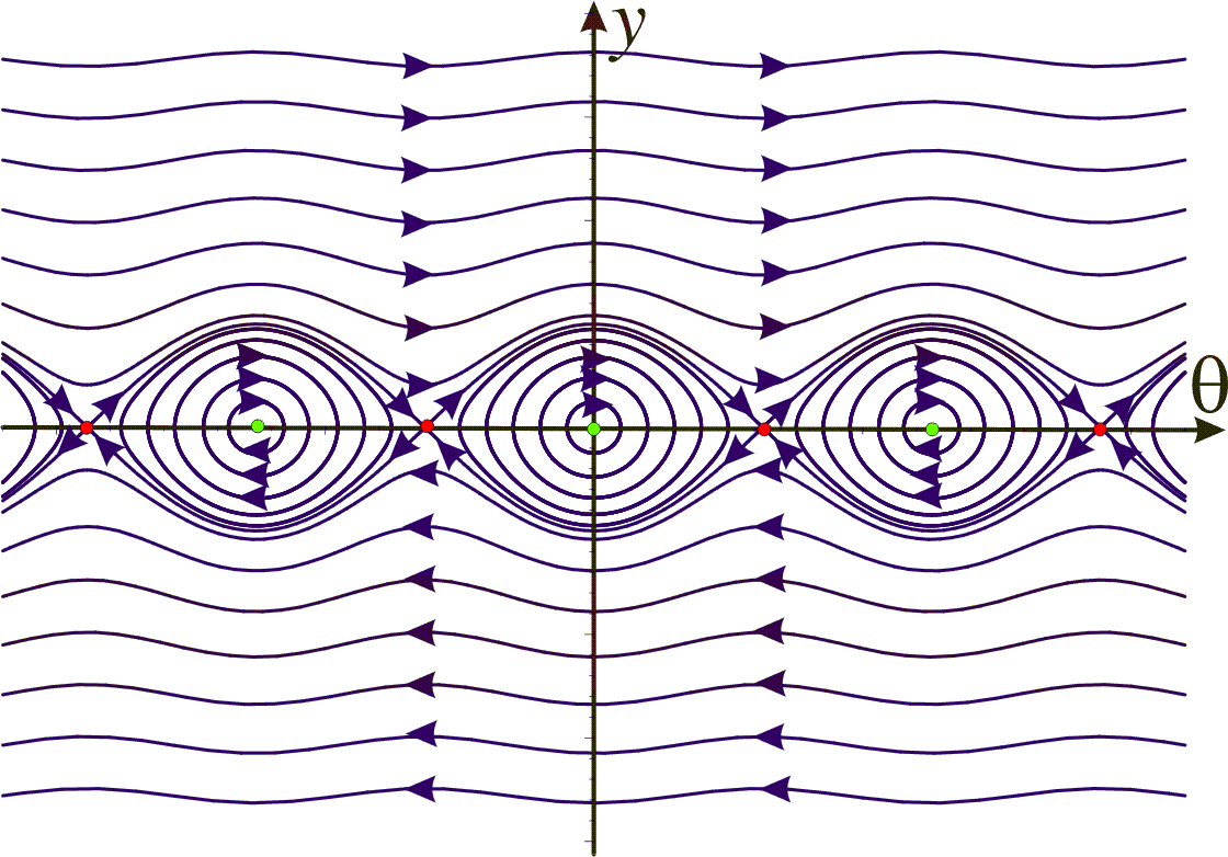
Here

are stable equilibrium points (colored green in the phase portrait) and

unstable equilibrium points (colored red in the phase portrait).
Example 6: Van der Pols equation

can be written as
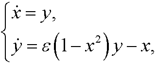
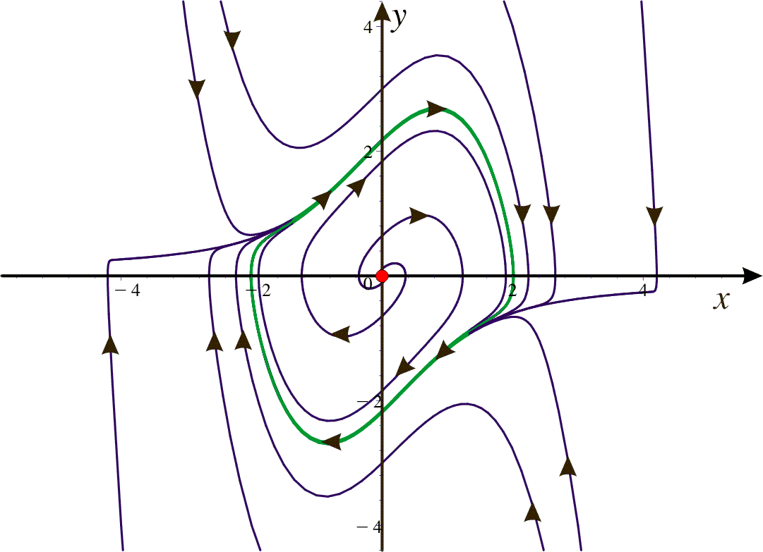
where ![]() is a (small) parameter. Here we have an (unstable) equilibrium point (0,0) (red color) and if we look at the phase portrait we see that we also have a limit cycle. This limit cycle (green color) is stable (all solutions in the neighborhood will be attracted to the limit cycle). We have plotted the phase portrait below for
is a (small) parameter. Here we have an (unstable) equilibrium point (0,0) (red color) and if we look at the phase portrait we see that we also have a limit cycle. This limit cycle (green color) is stable (all solutions in the neighborhood will be attracted to the limit cycle). We have plotted the phase portrait below for ![]() .
.
Example 7: Predators and prey, Volterra’s model.
There are two different species of fish in a lake: A (prey), that feeds off sea weeds (which is abundant) and B (predator), that feeds off the prey A.
The more prey A we have, the higher growth of A since the sea weed can be supposed to be enough to feed all. On the other hand, the growth of A is limited by the number of encounters between A and B, since they lead to that A being eaten. The more predators B, the lower growth of B since then we will have bigger concurrence about the prey A. On the other hand, the growth increases with the number of encounters between A and B, since Bgets food this way. If conclude the above reasoning, we get Volterra‘s model
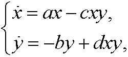
where a, b, c, d are positive constants, x=x(t) the population of A and y=y(t) the population of B at time t.
We get the equilibrium points by solving the system
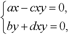
that is
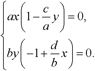
We have two possibilities for both equations to become zero. Either we have (x,y)=(0,0) or we have (x,y)=(b/d,a/c). If we draw the phase portrait we see thatthe first point is unstable while the second is stable.
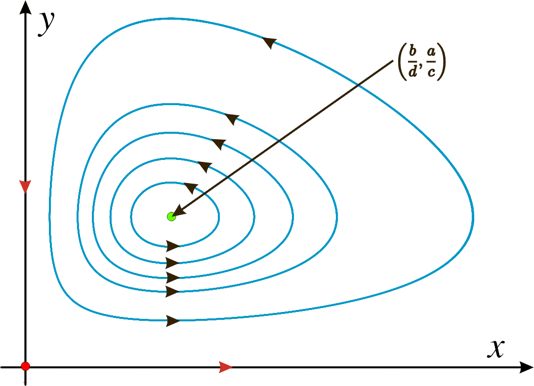
This model is useful to explain many well known biological phenomena when we have some kind of competition between different animals, for instance foxes and rabbits.