Again consider the system

The equilibrium point obviously is (0,0). Let ![]() and
and ![]() be the eigenvalues to the matrix A. We have the following different possibilities:
be the eigenvalues to the matrix A. We have the following different possibilities:
1) If
Let
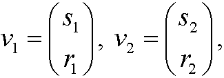
be the eigenvectors belonging to the corresponding eigenvalues ![]() and
and ![]() . Then the general solution of the system above is
. Then the general solution of the system above is

We again have a number of possibilities:
i) c2=0, c1>0: x(t) is a curve along l1+ (away from origo for increasing t).
ii) c2=0, c1<0: x(t) is a curve along l1– (away from origo for increasing t).
iii) c1=0, c2>0: x(t) is a curve along l2+ (away from origo for increasing t).
iv) c1=0, c2<0: x(t) is a curve along l2– (away from origo for increasing t).
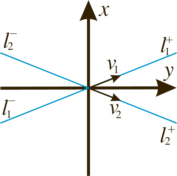
v) neither c1 nor c2 are zero. Then for
we have
hence
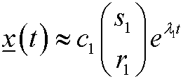
for large (in absolute value) negative t. In particular we have that

When
we have

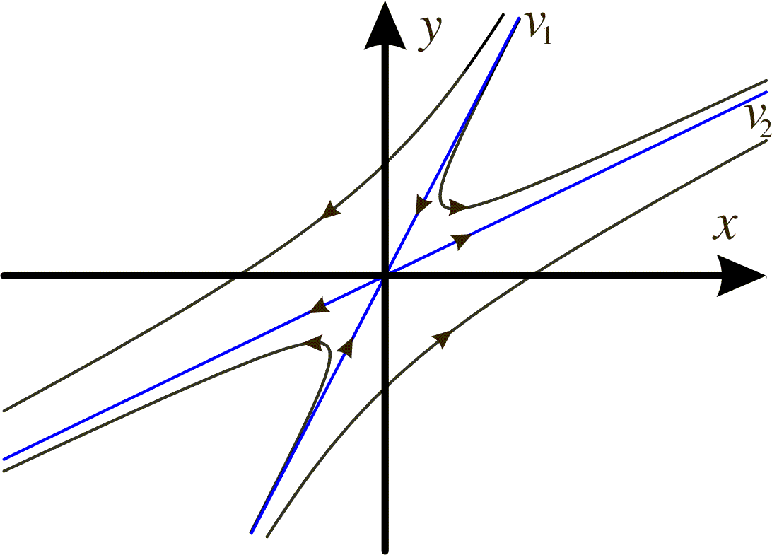
for large positive t. Hence x(t) diverges to infinity with a slope asympotically v2 as t goes to (positive) infinity. This means that (0,0) is an unstable node. The lines defined by the eigenvectors v1 and v2 are called separatrices. The behavior is shown below in the phase portrait.
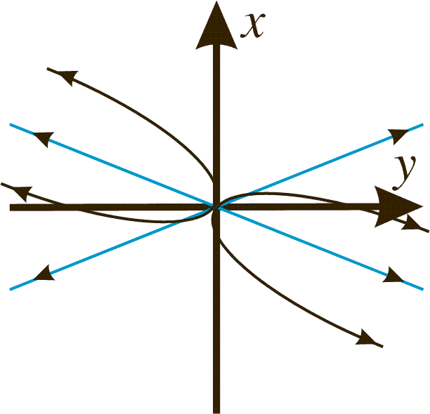
2) If
In the same way as above we realize that (0,0) is a stable node. The phase portrait looks the same but with reversed arrows.
3) If
We have the following possibilities:
i) c2=0, c1>0: x(t) is a curve along l1+ (towards origo for increasing t).
ii) c2=0, c1<0: x(t) is a curve along l1– (towards origo for increasing t).
iii) c1=0, c2>0: x(t) is a curve along l2+ (away from origo for increasing t).
iv) c1=0, c2<0: x(t) is a curve along l2– (away from origo for increasing t).
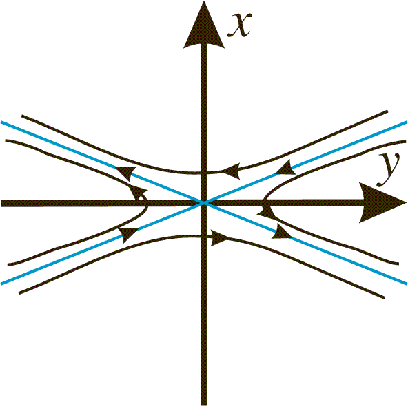
We have a saddle point. See the phase portrait below.
4) If
We have two cases:
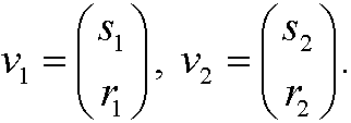
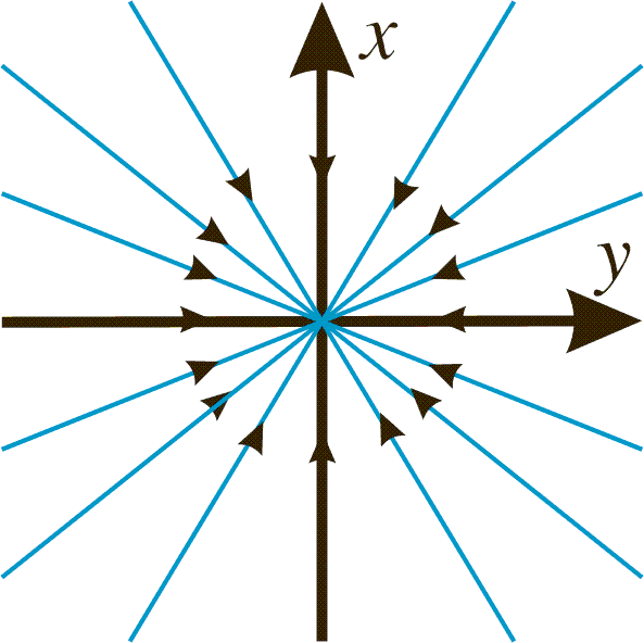
a) We have two linearly independent eigenvectors
Then we can write the solution

where a1 and a2 are arbitrary. This means that every curve is a halfline towards origo. See the phase portrait below.
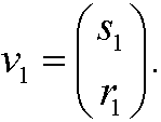
b) We only have one eigenvector
Then the solution on the form

where the vector
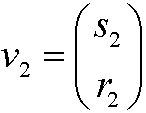
satisfies

For large t this means that the solution is
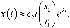
In this case the phase portrait will look like this.
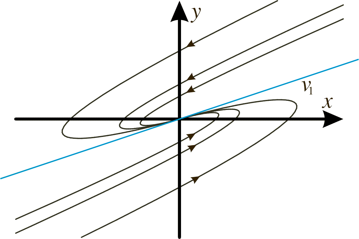
Both these cases are examples of a stable node.
5) If
This case is analogous to case 4) above, but with reversed arrows; (0,0) is an unstable node.
6) If
By using similar arguments as in Example 9 we realize that the real solutions are
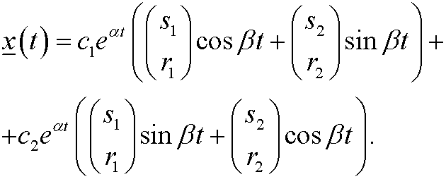
Three cases:
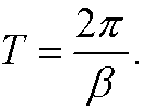
i) ![]() : Then x(t) and y(t) are periodic with period
: Then x(t) and y(t) are periodic with period
The point (0,0) is a center.
ii) ![]() : The amplitude of x decreases and we thus have a stable spiral.
: The amplitude of x decreases and we thus have a stable spiral.
iii) ![]() : The amplitude of x increases and we thus have an unstable spiral.
: The amplitude of x increases and we thus have an unstable spiral.

Example 10: Consider the system

The coefficient matrix
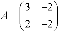
has the characteristic equation

and thus the eigenvalues
This corresponds to case 3) above and we conclude that (0,0) is an unstable saddle point. The eigenvectors are obtained by solving the linear equation system:

Eigenvalue 1:
implies that
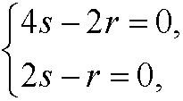
that is, the corresponding eigenvector is
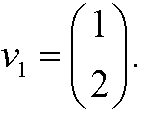
Eigenvalue 2:
implies that
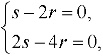
that is, the corresponding eigenvector is
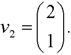
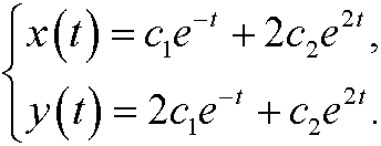
The general solution of the system thus is

that is
The eigenvectors define the directions of the separatrices.
Example 11: Consider the system
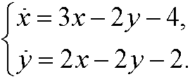
Here we have the critical point (2,1). We make the change of variables x1=x-2 and y1=y-1 and rewrite the system as
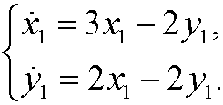
By using the result from example 10 above we see that the point (2,1) is an unstable saddle point and that the solution to the original system is

We get the phase portrait by taking that from example 10 and move it two steps in the x-direction and one step in the y-direction.
In the same way as in Example 11 we may instead study the more general system

The equlibrium point is here (a0,b0). By making the change of variables x1=x-a0 and y1=y-b0 we can transfer the system to the ones studied above with equilibrium point (0,0).